We were faced with an important question when working on Project Qian: Since cryptocurrencies have difference risk, how to quantify their risk?
Log return of an asset, as we all know, is an important measure of an underlying cryptocurrency. Then what about we simply measure the risk of an asset by its annualised log return? The lower, the riskier. Sounds right, but something is not right. But then again, how do we define ‘the risk of an cryptocurrency asset’?
We defined the risk of an underlying asset as follows: the proportion you might lose with a given probability within a given time period, given normal market conditions, when you invest in that asset. The larger the aforementioned proportion, the riskier the underlying asset.
In our case, we are concerned with the proportion that one might lose at most, given 99% certainty, within one hour, given normal market conditions.
We use the hourly price data for Ethereum as an example.
Question #1: is there any correlation as to the rise and fall of the underlying asset?
Technically speaking, is there any autocorrelation on the annualised return of the underlying asset? The result is:
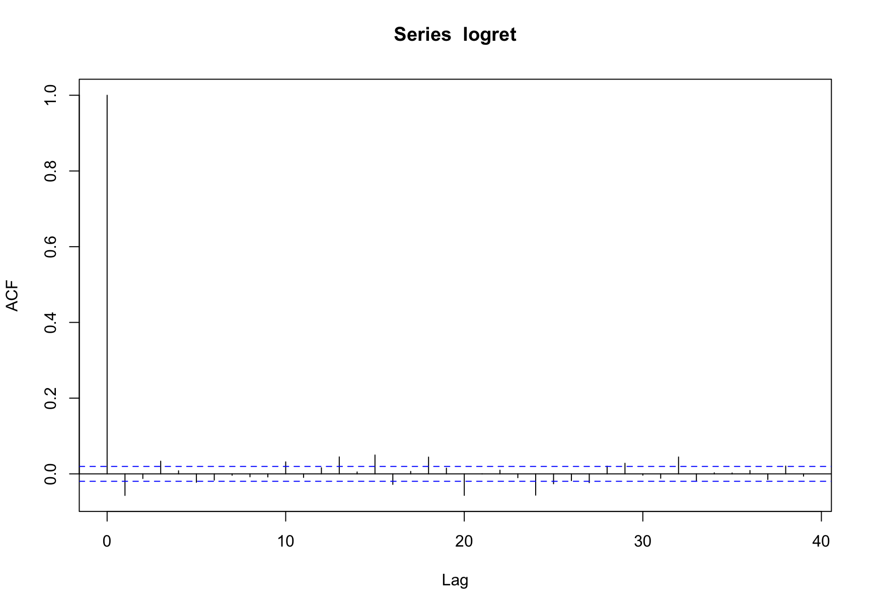
As you can see, the autocorrection is weak, which means that a surge or drop in price make little indication that it will move in the same direction in the next time interval.
It makes sense because if the rise and fall of an asset in a given interval indicated the direction of the next, then millionaires world be everywhere.
As there is little correction as to the return of the underlying asset, what about the absolute value of it?

It turns out that there is significant autocorrection indeed. It makes sense because in reality, high volatility tends to be followed by high volatility, and low volatility tends to be followed by low volatility.
This is what brings us to the generalised autoregressive conditional heteroskedasticity model, or GARCH for short.
To make use of the model, we still need to know the distribution of the logarithmic return of the underlying asset.
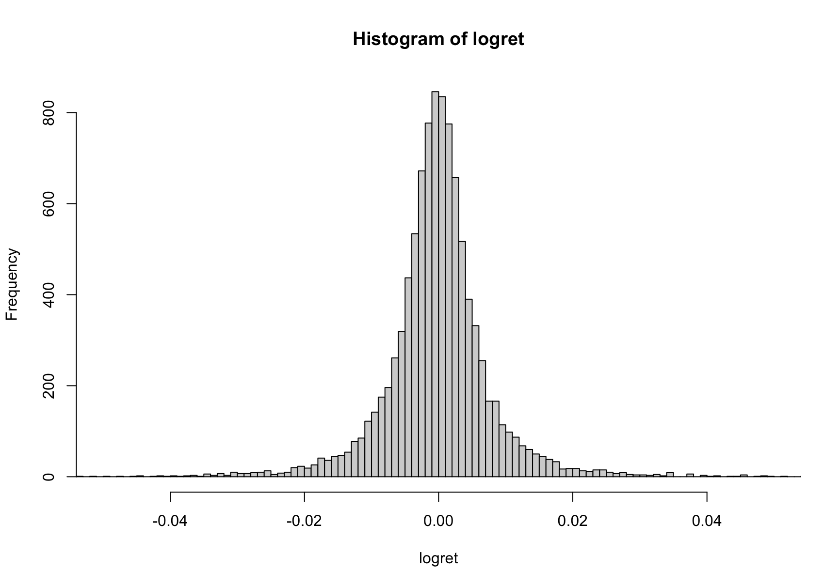
It may looks like a normal normal distribution. It really is abnormal. A Jarque-Bera test rejects its normality. It is actually a Student’s t distribution.
Thus, we are going to explain our data with the GARCH(1, 1) - Student’s t model:
(1) r_t = a_0 + 𝜎_t ^ 2 * 𝜀_t
(2) 𝜎_t ^ 2 = 𝛼_0 + 𝛽_1 * 𝜎_{t -1} ^ 2 + 𝛼_1 * 𝜀_{t-1} ^ 2
(3) 𝜀_t ~ t(𝜈) / sqrt(𝜈 / (𝜈 - 2))
In which:
- r_t is the return series with time varying volatility
- a_0 is the expected return, which is typically very close to zero
- 𝜎_t ^ 2 * 𝜀_t is the unexpected return
- 𝜎_t ^ 2 is the time varying predictable variance
- 𝜀_t is the Student’s t distributed residual